9 Modelling DBH x Height
9.1 Introduction
Permanent plot data lack total height, a critical variable for accurately estimating biomass. We obtained total heights for a subset of trees using LiDAR data (see Chapter 7). Additionally, we have other Forest Inventories conducted in the Jamari National Forest that include both DBH and total height.
We will use these data to model the DBH–Total Height relationship and derive a locally adjusted allometric equation to estimate the total height of trees in the permanent plot dataset. By combining total height with DBH, we expect to achieve more accurate biomass estimates for the permanent plots.
The modelling pipeline was developed by Sylvain Schmidt.
9.2 Lecture
- About tree height allometry: Molto et al. (2014)
- TALLO database: Jucker et al. (2022)
cmdstanrinstallation: https://mc-stan.org/cmdstanr/articles/cmdstanr.htmlstanprogramming: https://mc-stan.org/
9.3 Setup
You only need the tidyverse package for table manipulation and figures preparation, cmdstanr, brms, and bayesplot for Bayesian statistics.
9.4 Data
Data are tree hight and diameter from the TALLO database (Jucker et al. 2022) itself using dos-Santos et al. (2022) data for Jamari. Longitude and latitude are in degrees, so 1 degree is about 110 km at the equator, and we use a buffer of 10km. We have a total of 974 individuals and 134 species.
Code
lon <- -62.99
lat <- -9.11
buffer <- 10/110
data <- read_csv("data/forest_inventory/tallo.csv") %>%
  filter(longitude >= lon-buffer, longitude <= lon+buffer,
          latitude >= lat-buffer, latitude <= lat+buffer) %>%
  mutate(species = paste(genus, species)) %>%
  select(tree_id, species, height_m, stem_diameter_cm)
ggplot(data, aes(stem_diameter_cm, height_m)) +
  geom_point(aes(col = species), alpha = 0.25) +
  theme_bw() +
  geom_smooth(se = FALSE) +
  scale_color_discrete(guide = "none") +
  xlab("diameter (cm)") + ylab("height (m)") +
  ggtitle(paste(nrow(data), "individuals"),

          paste(unique(data$species) %>% length(),
                "species"))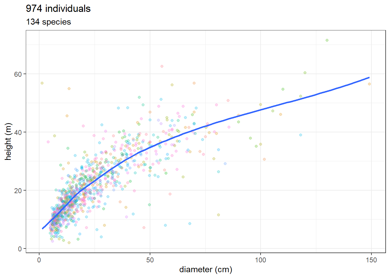
Let’s see if data from dos-Santos et al. (2022) are the same. Filter only tree (type == “O”) and alive (dead == “A”).
Code
dos_santos <- list.files("data/forest_inventory",
                          pattern = "^JAM.*\\.csv$",
                          full.names = T)

dos_santos_df <- dos_santos %>%
                        purrr::map_df(~ read_csv(.x,
                                      show_col_types = FALSE,
                                      col_types = cols(.default = col_character()))) %>%
                               filter(type == "O" ,
                                      dead == "A",
                                      !is.na(transect))


ggplot(dos_santos_df, aes(as.numeric(DBH), as.numeric(Htot))) +
  geom_point(aes(col = scientific_name), alpha = 0.25) +
  theme_bw() +
  geom_smooth(se = FALSE) +
  scale_color_discrete(guide = "none") +
  xlab("diameter (cm)") + ylab("height (m)") +
  ggtitle(paste(nrow(dos_santos_df), "individuals"),
          paste(unique(dos_santos_df$scientific_name) %>% length(),
                "species"))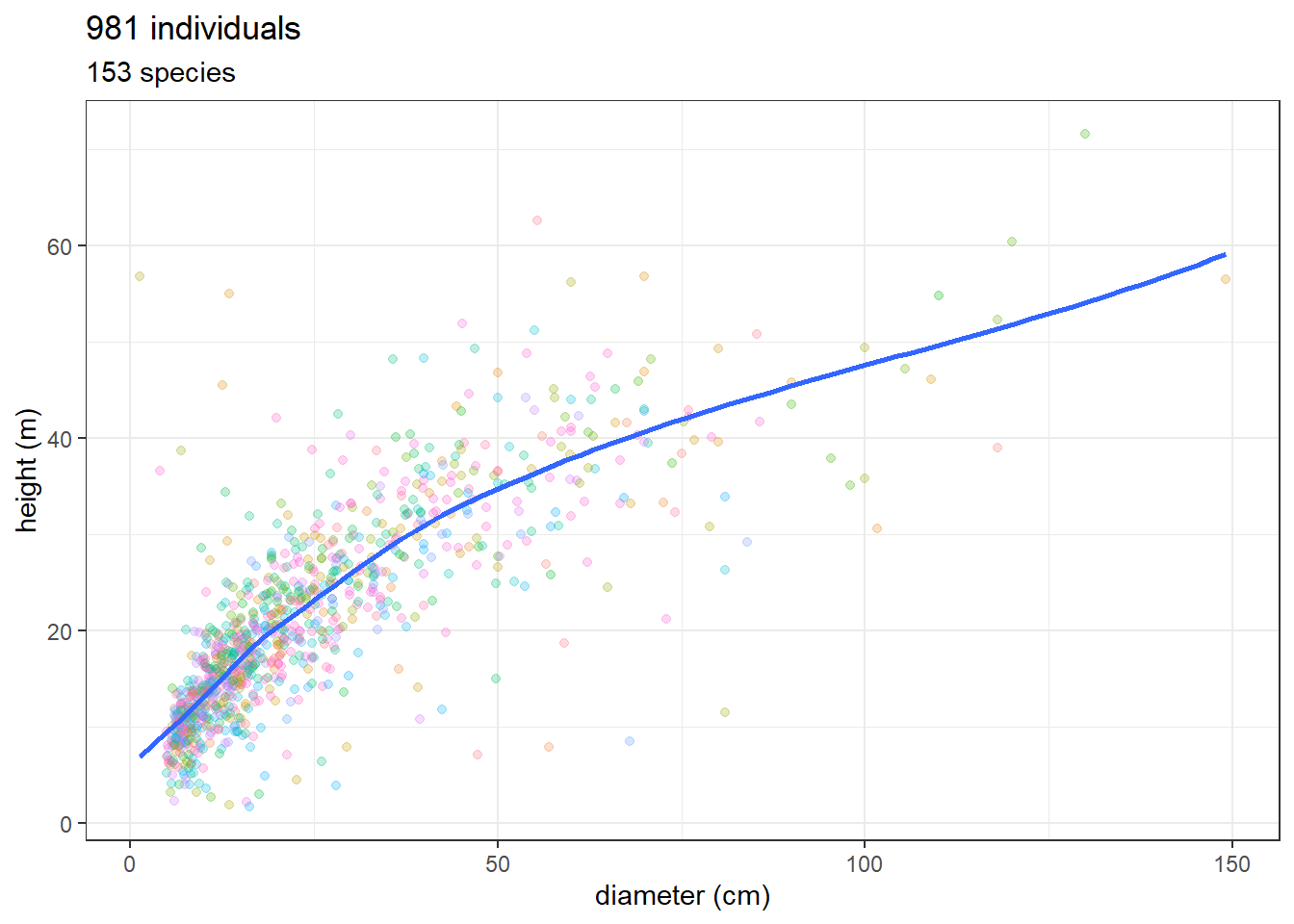
We will harmonize scientific names using ‘check_names’ function of the florabr package. check_names need input names So we will remove any “cf.” from the names, and also any words in parentheses. Then we will extract only genus and epithet (with get_binomial). Some species can’t be corrected with check_names. We will have to correct them mannualy.
Code
###########################################################################################

# Clean scientific names:
  # 1. Convert to UTF-8 because of the value on the row 340 - \xa0 = non-breaking space (NBSP)
  # 2. Remove "cf."
  # 3. Remove anything under parentheses.

dos_santos_df$scientific_name <- iconv(
  dos_santos_df$scientific_name,
  from = "",
  to = "UTF-8",
  sub = " "
)

  dos_santos_df$nome_corrigido <- trimws(
                                  gsub("\\s*cf\\.\\s*|\\([^)]*\\)",
                                       " ",
                                       dos_santos_df$scientific_name,
                                       ignore.case = T
                                       )
                                     )

  # Get the binomial name (epithet + genus)

  dos_santos_df$nome_corrigido <-  get_binomial(dos_santos_df$nome_corrigido)

if (!file.exists("data/taxo/dos_santos_2022_florabr_taxo.rds")) {


  # Check names with florabr

  floraBR <- load_florabr("C:/Gustavo/Doutorado/Dados/Taxo_databases/florabr")

   res_florabr <- check_names(data = floraBR,
                                     max_distance = 0.1,
                                     species = dos_santos_df$nome_corrigido,
                                     parallel = T,
                                     ncores = 12,
                                     progress_bar = T
                                       )

   # Resolve some species mannualy

   write.csv(res_florabr$input_name[res_florabr$Spelling == "Not_found"],
             file = "data/taxo/manually_corrected_species_dos_santos_2022.csv")

   # Hymenaea capanema
   # https://www.gbif.org/pt/species/7296249
   res_florabr$acceptedName[res_florabr$input_name == "Rinorea passoura"] <- "Rinorea pubiflora"

   saveRDS(res_florabr, "data/taxo/dos_santos_2022_florabr_taxo.rds")
                                                } else {
   res_florabr <- readRDS("data/taxo/dos_santos_2022_florabr_taxo.rds")
                                                       }

res_florabr_unique <- res_florabr %>%
  distinct(input_name, .keep_all = TRUE)

dos_santos_df <- dos_santos_df %>%
  left_join(
    res_florabr_unique %>%
      select(input_name, acceptedName),
    by = c("nome_corrigido" = "input_name")
  ) %>%
  mutate(
    nome_florabr = case_when(
      # keep name when second word is "sp.", since florabr assign a random name in these cases
      str_detect(nome_corrigido, "^\\S+\\s+sp\\.$") ~ nome_corrigido,
      TRUE ~ acceptedName
    )
  ) %>%
  select(-acceptedName)


sp <- read.csv("data/taxo/manually_corrected_species_dos_santos_2022.csv",
stringsAsFactors = FALSE)

text <- {
species <- sp$x
species <- species[!is.na(species)]

if (length(species) > 0) {
paste(
"Species corrected manually (n =",
length(species),
"):",
paste(species, collapse = ", ")
)
} else {
"No species required manual correction."
}
}Species corrected manually (n = 1 ): Rinorea passoura
Let’s see Brazilian National Forest Inventory data on Flona de Jamari. We will load the full inventory from Rondônia state and then we filter only the four plots inside Flona de Jamari (plots RO_74, RO_75, RO_95, RO_96)
Code
ifn_data <- read.csv2("data/forest_inventory/IFN_DAP10_Rondônia_disp-set2025.csv",
                      dec = ",")

ifn_data_jamari <- subset(ifn_data,
                          ua == "RO_74" | ua == "RO_75" | ua == "RO_95" | ua == "RO_96")

ggplot(ifn_data_jamari, aes(as.numeric(dap), ht)) +
  geom_point(aes(col = scientific_name), alpha = 0.25) +
  theme_bw() +
  geom_smooth(se = FALSE) +
  scale_color_discrete(guide = "none") +
  xlab("diameter (cm)") + ylab("height (m)") +
  ggtitle(paste(nrow(ifn_data_jamari), "individuals"),
          paste(unique(ifn_data_jamari$scientific_name) %>% length(),
                "species"))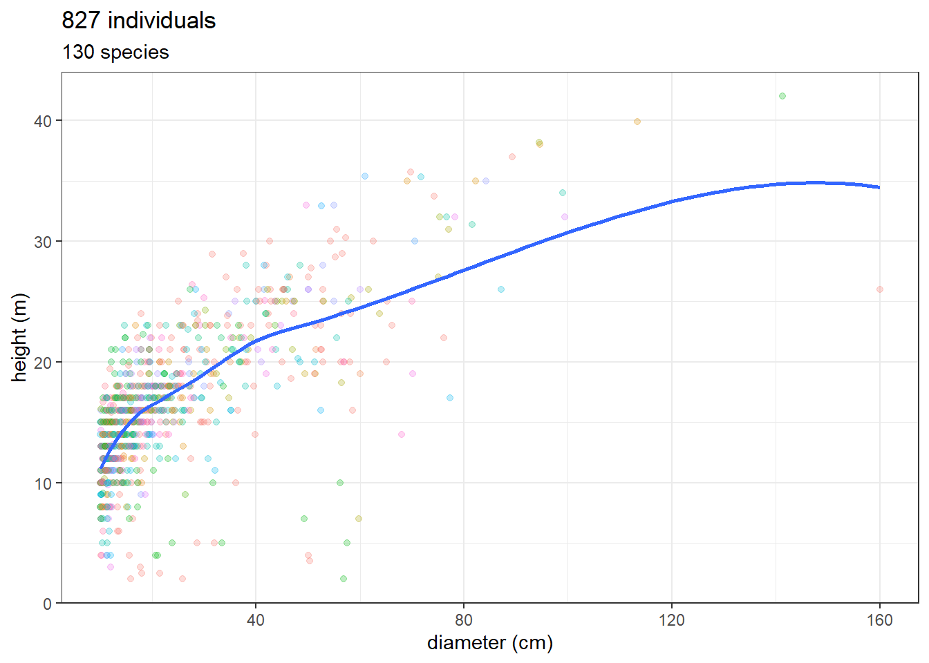
We will harmonize scientific names using ‘check_names’ function of the florabr package. check_names need input names We will use ´genus´ and epithet columns, and assign “NI” for non identified trees. Some species can’t be corrected with check_names. We will have to correct them mannualy.
Code
###########################################################################################

ifn_data_jamari <- ifn_data_jamari %>%
                           mutate(
                              nome_corrigido = case_when(
                              !is.na(genus) & genus != "" & !is.na(specific_epithet) & specific_epithet != "" ~
                              paste(genus, specific_epithet),

                              !is.na(genus) & genus != "" ~
                              paste0(genus, " sp."),

                              TRUE ~ "NI"
                                                        )
                                  )


#####
#  Loop
#####

if (!file.exists("data/taxo/ifn_data_jamari_florabr_taxo.rds")) {


  # Check names with florabr

  floraBR <- load_florabr("C:/Gustavo/Doutorado/Dados/Taxo_databases/florabr")

   res_florabr <- check_names(data = floraBR,
                                     max_distance = 0.1,
                                     species = ifn_data_jamari$nome_corrigido,
                                     parallel = T,
                                     ncores = 12,
                                     progress_bar = T
                                       )

   # Resolve some species mannualy

   write.csv(res_florabr$input_name[res_florabr$Spelling == "Not_found" & res_florabr$input_name == "^\\S+\\s+sp\\.$"],
             file = "data/taxo/manually_corrected_species_ifn_data_jamari.csv")

   saveRDS(res_florabr, "data/taxo/ifn_data_jamari_florabr_taxo.rds")
                                                } else {
   res_florabr <- readRDS("data/taxo/ifn_data_jamari_florabr_taxo.rds")
                                                       }

res_florabr_unique <- res_florabr %>%
  distinct(input_name, .keep_all = TRUE)

ifn_data_jamari <- ifn_data_jamari %>%
  left_join(
    res_florabr_unique %>%
      select(input_name, acceptedName),
    by = c("nome_corrigido" = "input_name")
  ) %>%
  mutate(
    nome_florabr = case_when(
      # keep name when second word is "sp.", since florabr assign a random name in these cases
      str_detect(nome_corrigido, "^\\S+\\s+sp\\.$") ~ nome_corrigido,
      TRUE ~ acceptedName
    )
  ) %>%
  select(-acceptedName)


ifn_data_jamari$nome_florabr[ifn_data_jamari$nome_corrigido == "NI"] <- "NI"

sp <- read.csv("data/taxo/manually_corrected_species_ifn_data_jamari.csv",
stringsAsFactors = FALSE)

text <- {
species <- sp$x
species <- species[!is.na(species)]

if (length(species) > 0) {
paste(
"Species corrected manually (n =",
length(species),
"):",
paste(species, collapse = ", ")
)
} else {
"No species required manual correction."
}
}No species required manual correction.
Merging two datasets (dos-Santos et al. (2022) and IFN) in a standardized data frame.
Code
df1_clean <- dos_santos_df %>%
  select(nome_florabr, DBH, Htot) %>%
  mutate(DBH = as.numeric(DBH),
         Htot = as.numeric(Htot),
         source = "dos_santos") %>%
  rename(
    dbh = DBH,
    total_height = Htot
  )

df2_clean <- ifn_data_jamari %>%
  select(nome_florabr, dap, ht) %>%
  mutate(dap = as.numeric(dap),
         source = "IFN") %>%
  rename(
    dbh = dap,
    total_height = ht
  )


jam_for_inv <- bind_rows(df1_clean, df2_clean)


ggplot(jam_for_inv, aes(dbh, total_height)) +
  geom_point(aes(col = nome_florabr), alpha = 0.25) +
  theme_bw() +
  geom_smooth(se = FALSE) +
  scale_color_discrete(guide = "none") +
  xlab("diameter (cm)") + ylab("height (m)") +
  ggtitle(paste(nrow(jam_for_inv), "individuals"),
          paste(unique(jam_for_inv$nome_florabr) %>% length(),
                "species"))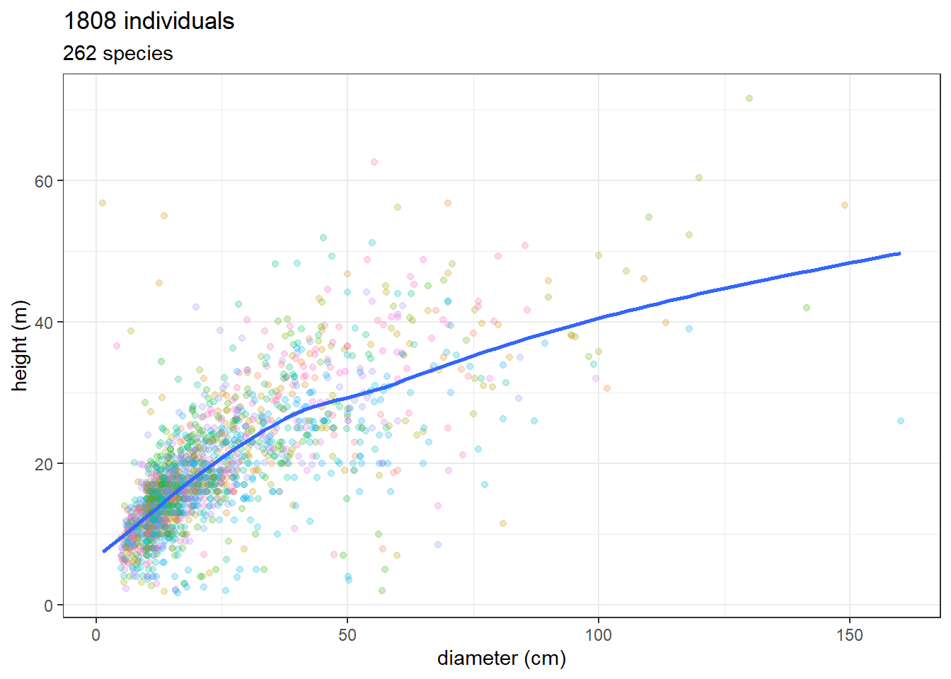
Now let’s load our commercial inventory dataset with Lidar derived height (see Chapter 7) and merge with the previous dataset.
Code
if100_lidar <- read.csv("output/tree_height/all_tables.csv")
if100_lidar <- if100_lidar %>%
                    filter(!is.na(z_lidar)) %>%
                    select(c("nome_florabr",
                             "DAP",
                             "z_lidar")) %>%
                    rename(dbh = DAP,
                           total_height = z_lidar) %>%
                    mutate("source" = "if100_lidar")

jam_for_inv <- bind_rows(jam_for_inv, if100_lidar)

ggplot(jam_for_inv, aes(dbh, total_height)) +
  geom_point(aes(col = nome_florabr), alpha = 0.25) +
  theme_bw() +
  geom_smooth(se = FALSE) +
  scale_color_discrete(guide = "none") +
  xlab("diameter (cm)") + ylab("height (m)") +
  ggtitle(paste(nrow(jam_for_inv), "individuals"),
          paste(unique(jam_for_inv$nome_florabr) %>% length(),
                "species"))
`geom_smooth()` using method = 'gam' and formula = 'y ~ s(x, bs = "cs")'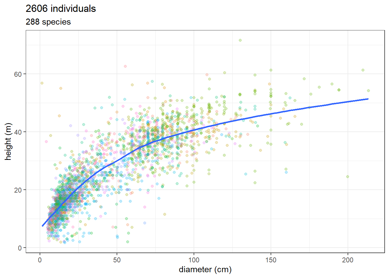
9.5 Model
We model tree height \(h\) in function of tree diameter \(d\) as:
\[ h \sim logN( \frac{h_{max}\times d}{a + d} , \sigma) \]
with \(h_{max}\) the maximum tree height and \(a\).
9.6 Example with cmdstanr
Code
data {
  int<lower=0> N;
  vector[N] h;
  vector[N] d;
}
parameters {
  real<lower=1, upper=100> hmax;
  real<lower=0> a;
  real<lower=0> sigma;
}
model {
  log(h) ~ normal(log(hmax*d ./ (a+d)), sigma);
}
Code
 variable    mean  median   sd  mad      q5     q95 rhat ess_bulk ess_tail
    lp__  1603.45 1603.77 1.22 0.97 1601.02 1604.74 1.00     1413     1813
    hmax    52.62   52.56 0.99 1.01   51.08   54.31 1.00     1471     1692
    a       37.15   37.10 1.23 1.24   35.23   39.20 1.00     1492     1600
sigma 0.33 0.33 0.00 0.00 0.32 0.34 1.00 2153 1699`stat_bin()` using `bins = 30`. Pick better value `binwidth`.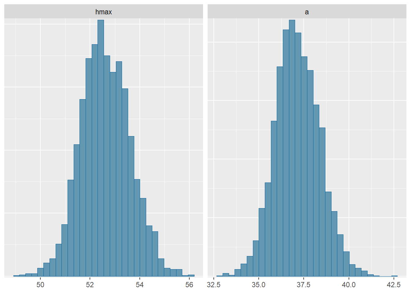
Code
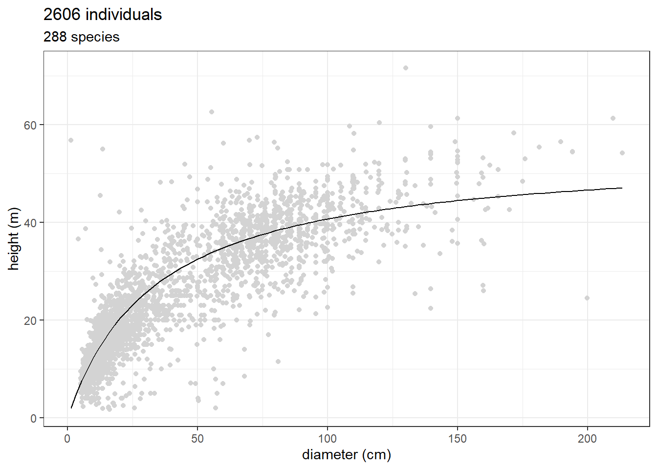
ggplot(jam_for_inv, aes(dbh, total_height)) +
  geom_point(col = "lightgrey") +
  stat_function(fun = function(x) 54.50*x/(33.90+x)) +
  theme_bw() +
  xlab("diameter (cm)") + ylab("height (m)") +
  ggtitle(paste(nrow(jam_for_inv), "individuals"),
          paste(unique(jam_for_inv$nome_florabr) %>% length(),
                "species"))